Operation Overpass: Part 3 - Covert QL

Initiate Your Journey into the Shadows of OSM Intelligence.

Welcome back to our digital command centre. As we continue to decode the secrets of Overpass QL for OSINT missions, it’s crucial to reflect on the groundwork laid in Article 2 of this series. If you’ve not yet mastered those basics, a strategic review at Operation Overpass: Part 2 - Covert QL is recommended.

Today, we escalate our operational techniques, honing in on individual elements within the vast data territories we navigate. We’ll refine our searches with precise keys, deploy the 'around' function for meticulous proximity reconnaissance, and initiate the use of MapCSS to bring clarity to our field maps. Though styling may seem a secondary concern, its simplicity belies a significant tactical advantage—clearly distinguishing between myriad data points on densely populated maps.

Ensure your digital toolkit is operational—Overpass Turbo will be our primary interface for today’s data maneuvers.

Prepare to dive deeper into the intelligence-gathering capabilities of Overpass QL. Let’s decode, discover, and dominate our digital landscape. Ready to advance? Let’s move out.

1. Targeting Individual Elements

Visualise our scenic target: the café captured in the image, a charming enclave nestled in the embrace of Sydney's vibrant historic architecture. This spot, which holds alfresco diners under the shade of broad umbrellas, becomes the focus of our digital reconnaissance.

Image Analysis - Cafe

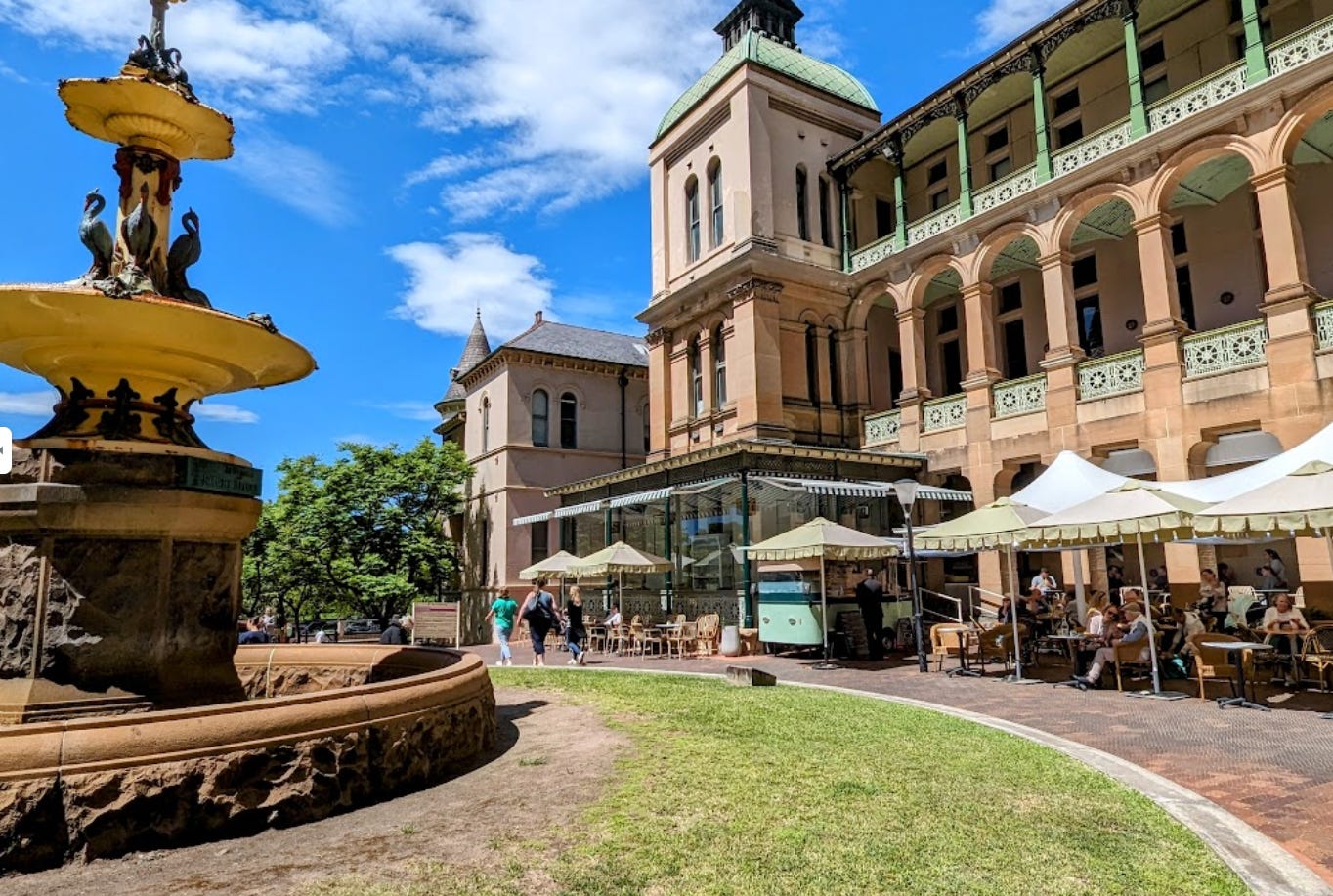
As we've ventured through the digital landscapes in our series, recall the indispensable OSM wiki map features highlighted in our initial guide. It's crucial now as we prepare to dissect this image through our queries.

Let's hone in on our target. Within the vast OSM database, our café is categorised as an 'amenity', a beacon for our search efforts in the digital sea of data. Here's the Overpass Turbo query we use to illuminate our target within the City of Sydney:

{{geocodeArea:Sydney City}}->.searchArea; 

( 
    nwr[amenity="cafe"](area.searchArea); 
    <; 
); 

out meta;

This query casts a wide net, sweeping through Sydney to snag every node, way, and relation tagged as a café. It's our initial broad stroke, mapping the terrain.

How We Constructed This Query:

1. We initiated with the {{geocodeArea:Sydney City}} to define our broad search area. This sets the geographic context of our query within Sydney.

2. The nwr[amenity="cafe"] part of the query is targeted, looking specifically for nodes, ways, and relations tagged as cafés.

3. The use of <; ensures that we gather all related data tied to these cafés, such as associated nodes for ways and relations.

4. out meta; ensures that the output includes all metadata, providing comprehensive details for each café entity.

As we further dissect this query, notice the use of brackets—round ‘( )’ and square ‘[ ]’. In the language of Overpass, QL is used to group elements or subqueries, which is essential for structuring complex queries. They can define the scope of a query part and control the execution order. Meanwhile, square brackets filter elements based on certain criteria. These criteria can include tags, which are key-value pairs attached to elements in OSM to describe the properties of the object, in this case, cafés.

However, running this query floods us with data, a deluge of nodes, each representing potential café locations. For a field operative, sifting through this vast array manually is impractical.

Query Link

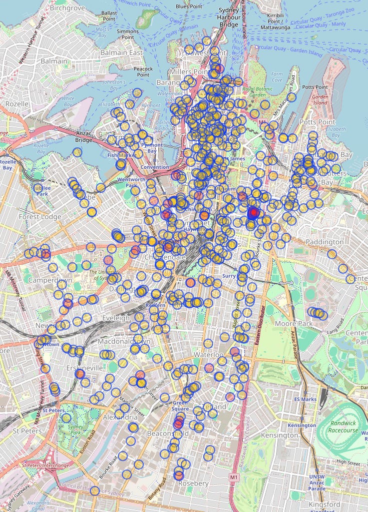
But, our first pass reveals too many potentials—the city is teeming with cafés. So, drawing from the image's hint of outdoor seating—a specific feature that can drastically narrow our search. We update our query to pinpoint only those cafés offering outdoor seating, as captured in our visual intel:

{{geocodeArea:Sydney City}}->.searchArea; 

(
    nwr[amenity="cafe"][outdoor_seating=yes](area.searchArea);
    <;
);

out meta;

How We Constructed This Refined Query: Here, we've introduced [outdoor_seating="yes"] to our filter criteria, narrowing our search to only those cafés that offer outdoor seating, as depicted in our image. This criterion significantly reduces the data clutter by filtering out cafés without outdoor facilities, aligning our digital search with our visual intelligence.

Query Link

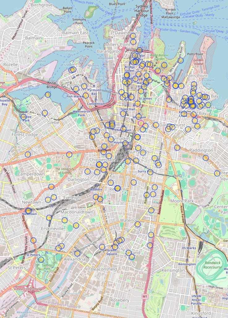
This tailored approach slashes through the surplus, yielding a more manageable list of locations. Each data point now more closely reflects the characteristics of our café in the image. Yet, while we've refined our focus effectively, achieving a sharp edge in our data blade, we may still need to expand or further specify our parameters.

The subsequent step in our strategy involves either adding more nuanced keys to these cafés to tighten the net further or extending our scope to include elements ‘around’ the café, such as nearby landmarks or additional amenities that could provide further context or draw a more detailed map of the area's social geography. This dual approach ensures that we are not just collecting dots on a map, but weaving a tapestry of interconnected data that can lead to richer, actionable insights.

2. Using the ‘around’ Function

The ‘around’ function opens up a new dimension in our digital explorations. It is particularly useful for proximity searches that require us to look beyond a single point of interest. For this exercise, let's expand our focus from the café to include the nearby captivating fountain visible in our image.

Imagine a scenario where knowing the relationship between cafés and nearby amenities, like fountains, could provide crucial context or simply enhance our understanding of the area. Here’s how we adjust our query to include these elements:

{{geocodeArea:Sydney City}}->.searchArea;   	

nwr[amenity="cafe"][outdoor_seating=yes](area.searchArea)->.myCafe;

(
    nwr[amenity="fountain"](around.myCafe:20)->.fountain;
    nwr[amenity="cafe"][outdoor_seating=yes](around.fountain:20);
    <;
);

out meta;

How We Constructed This Query:

1. We begin by setting the geographic stage with {{geocodeArea:Sydney City}} which defines our search area, tagged as .searchArea.

2. We identify and store our primary target, the café with outdoor seating, in a result set named .myCafe.

3. We then introduce a new element, the fountain, using nwr[amenity="fountain"](around.myCafe:20)->.fountain. This line searches for fountains within a 20-meter radius of our defined café set, .myCafe.

If we left that here, the Overpass API would only return fountains around the cafe but not the cafe itself. I also like to include the primary search element (the cafe) to provide more visual clarity in my searches.

4. So, we will assign -> our fountain element to a result set .fountain.

5. Now we will reintroduce our search for our cafe nwr[amenity="cafe"][outdoor_seating=yes] but only those cafes around 20 meters from fountains (around.fountain:20).

Query Link

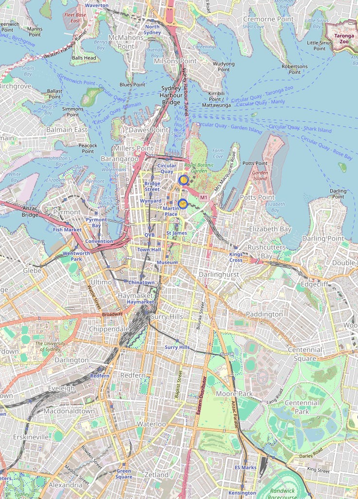
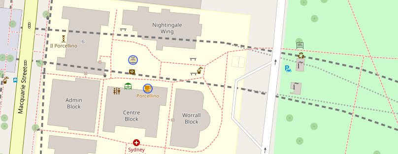
The execution of this query reveals an intricate dance of nodes where cafés and fountains play key roles. With four nodes returned—two fountains and two cafés—we gain a detailed snapshot of the immediate surroundings.

Surprisingly, the query’s efficiency in pinpointing our location without requiring extensive manual filtering is a testament to the power of precise element targeting and proximity functions in Overpass QL.

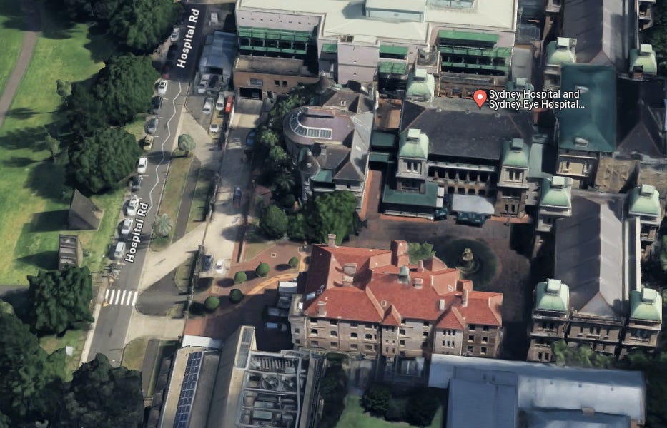
Zooming in on the southernmost location, I could say with high confidence that this is our location without even looking at Google Earth. We see a cafe and a fountain in a courtyard, two separate buildings, a park, and a plaque in front of the fountain. All these elements are visible within our original image.

Southernmost query results

Google sat image of cafe location.

---

I would now like to quickly touch on the styling of elements within the map. This is particularly helpful when trying to distinguish one element from the next. We always want to return and present data in a meaningful way, in a way that is quick to interpret.

3. Adding mapCSS Styles to Elements

Now, let's shift our focus to enhancing the visual presentation of our data on the map. The ability to clearly differentiate between elements such as train stations, cafes, and other points of interest is essential for effective data interpretation.

Let’s initiate a query aimed at locating a specific underground train station and surrounding cafes, serving as an excellent case study for applying styling:

{{geocodeArea:Sydney}}->.searchArea;

nwr[name="Martin Place Train Station"](area.searchArea)->.sydneyTrain;

(
	nwr[amenity="cafe"](around.sydneyTrain:70);
  	nwr[name="Martin Place Train Station"];
	>;
);

out meta;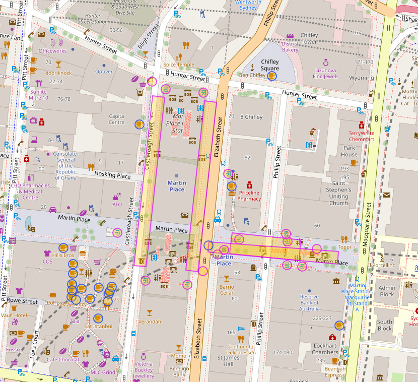

Query Link

Initially, without styling, the map presents all elements in the same colour, making it challenging to distinguish between them. Let's rectify this by integrating some MapCSS styling into our query. This styling sits at the end of your query below the output (out meta;).

In this instance, I want to define the styling of the train platforms (way), the entrances (node), and the cafes (node). We can do that exactly by using mapCSS styling.

{{style:
	way
  	{ color:black; width:4; opacity:1; }

        node[railway=subway_entrance]
	{ color:black; fill-color:white; }

	node[amenity=cafe]
	{ color:blue; fill-color:blue; }
}}

As you can see, styling is pretty self-explanatory, and we will explore this topic more in future articles. We define what element we want to style and then tell it how to style that element.

1. way elements, which could represent train platforms, are styled with a black color and a more substantial width for better visibility.

2. Subway entrances are marked distinctly with a black outline and white fill, making them stand out as specific points of entry to the subway.

3. Cafes are given a blue colour both for the outline and fill, immediately making them recognisable as distinct from other nodes and ways.

Here’s how our revised query looks with the styling applied:

{{geocodeArea:Sydney}}->.Sydney; 

nwr[name="Martin Place Train Station"]->.sydneyTrain; 

(
    nwr[amenity="cafe"](around.sydneyTrain:70); 
    nwr[name="Martin Place Train Station"]; 
    >; 
); 

out meta;

{{style:
	way
  	{ color:black; width:4; opacity:1; }

        node[railway=subway_entrance]
	{ color:black; fill-color:white; }

	node[amenity=cafe]
	{ color:blue; fill-color:blue; }
}}

Query Link

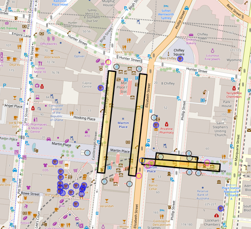
These styles enhance the map's clarity significantly, facilitating quick and effective data interpretation. This visual distinction helps anyone analysing the map to quickly identify and differentiate between the underground train entrances and the surrounding cafes.

---

I originally intended to present a deep dive into the reasons why you would use nwr over individual elements (node, way, relation) and vice versa within this lesson, but I will now present that information in the next article. So keep an eye out for that one.

Just to reiterate what we have learnt in this article:

1. how to search for an individual element, and

2. how to refine the particulars of an element and

3. how to search for an element within proximity of other elements, and finally

4. how to apply styling to elements within a query.

Within the next article, I will give you a greater understanding of when and when not use nwr element calls, I will also start to introduce ‘ways’ to search for such things as streets and bus or bike lanes as part of those streets, we will also again start returning elements along these ways, such as surveillance cameras, signs, power lines, bus stops etc.

I will leave you with a few exercises to work on to build your confidence in what we have learned to date. I am always happy to answer any questions, so feel free to leave a comment or message me, and I’ll endeavour to help you out.

Exercises

To solidify your understanding of these techniques, here are a few exercises:

1. Define a Search Area: Define other locations within the world. Practice with locations that are identical to somewhere else in the world. Sydney is a good example, as it resides in both Australia and Canada. How could you change the area location to search in Sydney, Canada?

2. Element Search: Write a query to locate all electric vehicle charging stations in the Sydney CBD area. Now, try to search for multiple elements.

3. Proximity Search: Use the 'around' function to find all parking lots within 500 meters of the Museum of Contemporary Art in Sydney. Then, experiment with various locations, distances and other elements.

Until next time, good luck and safe searches.

Journey deeper into the data labyrinth. See you on the other side.

-- ClearInsight

---